Exploring Starry Realms in the Milky Way with Gaia¶

Talk at PyDelhi x PyData Delhi : Meetup #46¶

Chetan Chawla¶

Co-Organizer @PyData Delhi; Tech Consultant @ZS; ex-Astrophysics Researcher @ASIAA¶

Open the Jupyter Notebook in Binder to try the tutorial yourself: bit.ly/gaia-notebook ¶

Or clone the repository to your local: github.com/chetanchawla/PyDD_Gaia_Talk ¶

1. Astronomy¶

Astronomy is the study of celestial objects and related phenomena
All objects in the space like stars (including our sun), planets (including planets hosted by other stars; exoplanets), moons (including moons hosted by exoplanets; exomoons), comets, galaxies, etc. are celestial objects

1.1 How do we do Astronomy?¶

The oldest records include people looking up at the sky with naked eyes and drawing what they see
They also made mathematical calculations using these celestial bodies, like making calendars, tracking their positions (astrometry), etc
Nowadays, we use data and simulations for astronomy.
The observational branch collects data by observing celestial objects through telescopes and then analyzes this data using Physics-Chem-Maths.
The theoritical branch uses the Physics-Chem-Maths to create analytical computer models and simulations for describing celestial objects and phenomena

Images Source: Wikipedia

1.2 Telescopes¶

Telescopes are instruments that are used to peer deeper into the space-time, than can be done with naked eye.
The different types of telescopes are classified based on the electromagnetic wavelengths they observe (Radio telescopes, IR telescopes, Visible telescopes).
These telescopes are often made big to increase their resolution and subsequently, how far we can look in the space.
Some are placed in observatories on Earth, while some travel/sit-in space to collect the data for us.

Images Source: Wikipedia

2. What is Gaia?¶

Space Mission led by the European Space Agency (ESA) to collect photometric (measurement of luminosity), spectroscopic (measurement of radiation intensity as a function of wavelength), and (primarily) astrometric (precise measurement of positions, distances and motions of stars and other astronomical bodies) data for several astronomical objects (mainly Milky Way stars)
Launched in 2013, and is expected to continue its mission until 2022
Aims for largest and most precise 3D space catalog of approx 1 billion astronomical objects at a precision of $\mu$as (micro-arcseconds) - mainly consisting of stars, but also planets, comets, asteroids and quasars among others.

Image Source: ESA: Gaia Operations

Image Source: Wikipedia

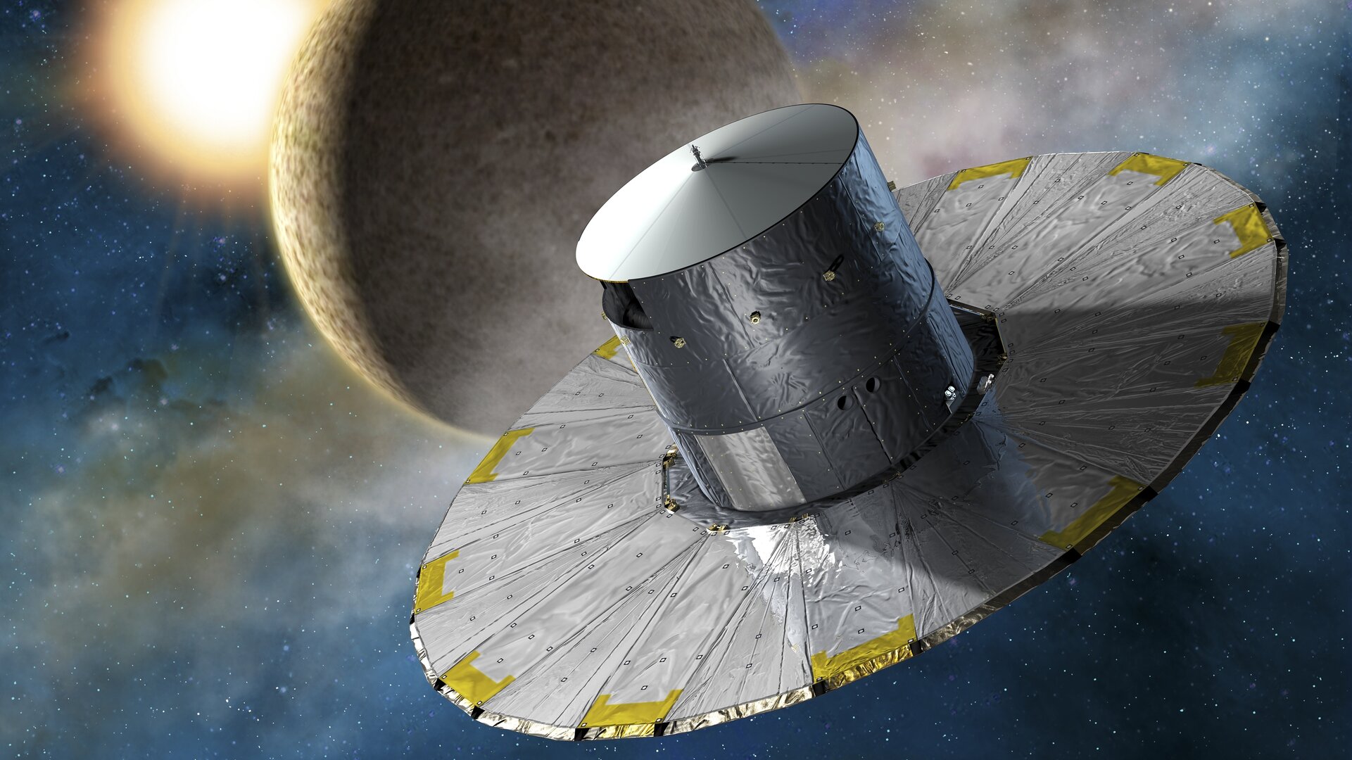
It is positioned on the second Lagrange point of the Earth-Sun system
It has two Three-Mirror Anastigmatic telescopes positioned at an angle of 106.5° to give wide fields of view and to give absolute astrometry.
It has a billion pixels in its camera (Giga-pixel)
It has the astrometric accuracy of a few microarcseconds (10-200 $\mu$as). It is about the size of an orange placed on the Moon as seen from Earth.
Gaia can be used for stellar astrophysics, positional and motion survey of a billion stars in the Milky Way, measuring distances of far away clusters using variable stars, potential exoplanet discoveries using astrometry(primarly) and transits, and spectroscopy of stars

Image Source: Manyworlds.space, C. Carreau/ESA

3. Gaia Data¶

Gaia Data primarily contains of -

Right Ascension (RA)
Declination (Dec)
Parallax
Radial Velocity (RV)
Proper Motion in terms of Right Ascension (pmra)
Proper Motion in terms of Declination (pmdec).

3.1 Right Ascension and Declination¶

They are the longitude and latitude to position an object in the celestial frame of reference
In other words, they are the celestial coordinates
They are calculated as positions in the plane of the sky.
Read more about them at https://skyandtelescope.org/astronomy-resources/right-ascension-declination-celestial-coordinates/.

Image Source: Wikipedia

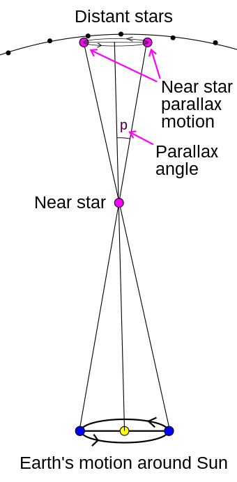
3.2 Parallax¶

The effect which causes an apparent shift in the position of an object with respect to a background when observed from two different points (separated by a distance called basis)
It is calculated as the semi-angle of inclination of these two different line of sights from the observation points to the object.
Image source and more at: https://en.wikipedia.org/wiki/Parallax

3.3 Radial Velocity¶

It is the velocity of an object in a direction away from or towards the Earth (observation point).
In a more general sense, it is the velocity between the object and the observation point in the direction of the radius connecting the point and the object

Image Source: F. Baron

3.4 Proper Motions (RA and Dec)¶

Proper Motion is the rate of angular drift in the plane of the sky or in a transverse direction
pmra and pmdec are the rates of change of the RA and Dec of an object in the sky respectively
Their resultant is also called the transverse velocity or total proper motion
The space velocity of an object is the resultant of the transverse velocity and the radial velocity

Images source and more at: Science at your doorstep

Parallax

4 Gaia Data Releases¶

Gaia data is made publicly available through periodic data releases (DRs).
Each Data Release has a richer data than the previous data release as Gaia covers the stars more times and adds new stars and objects as well.
We had two full releases (DR1 and DR2) until now, and an Early Data Release 3 (EDR3). We will be having DR3 in July'22

4.1 Gaia Archive¶

Gaia Archive is a remote server which hosts the publicly available DRs in the form of a database.
It also provides us an interface to query the data and manipulate it according to our needs on the server itself, without us having the need to download the data first on our local computers.
The Gaia archive can be found here: https://gea.esac.esa.int/archive/
The basic search can help us search data through a GUI. The advanced (ADQL) tab allows us to write our own complex queries in SQL-type language, called ADQL (Astronomical Data Query Language)

In [2]:

%%html
<div style="text-align:center;">
<iframe src="https://gea.esac.esa.int/archive//" width="960" height="540"></iframe>
</div>

4.2 Basic Search¶

Using Basic Search in Gaia Archive to fetch the first 2000 stars in 3 arcminutes radius circle around the globular cluster, Messier 5. We will then read this data in Python and plot the stars in a RA-Dec space

On the Basic search page
In the "Name" field, type in "Messier 5". It should resolve the name. This will center our search on M5, a globular cluster in the constellation Serpens.
To the right, put a "3" and then change the unit from "arc sec" to "arc min". This will tell the archive to search in a radius of 3 arcminutes around M5. There are 60 arcseconds in an arcminute, and 60 arcminutes in a degree.
Make sure that the "Search In" drop down says "gaiadr2.gaia_source". This specifies the data we want to use is frrom source of Gaia DR2
Click "Submit Query"
You'll see a table pop up with the first 20 results from the query. At the bottom, change "VOTable" to "csv" and click "Download results". This will download a csv to your computer with the queried data in it.

4.3 Taking the data to Python and Plotting it¶

In [3]:

# numpy, for math (numerical calculations)
import numpy as np
# pandas, for data handling
import pandas as pd
pd.set_option('display.max_columns', None) # Display all of the columns of a DataFrame
# matplotlib, for plotting
import matplotlib.pyplot as plt
# "Magic command" to make the plots appear *inline* in the notebook
%matplotlib inline

In [4]:

#Now we can read the csv file into a pandas dataframe
m5 = pd.read_csv('data/m5.csv') # I renamed my csv file to 'm5.csv' and put it in the the subfolder 'data'
#Checking the top few rows of the data and the number of rows and columns
print("(Rows, Columns) =", m5.shape)
m5.head()

(Rows, Columns) = (2000, 14)

Out[4]:

	source_id	ra	ra_error	dec	dec_error	parallax	parallax_error	phot_g_mean_mag	bp_rp	radial_velocity	radial_velocity_error	phot_variable_flag	teff_val	a_g_val
0	4421572868783602304	229.608260	0.451151	2.080235	0.755487	NaN	NaN	18.320505	NaN	NaN	NaN	NOT_AVAILABLE	NaN	NaN
1	4421573315458434816	229.661337	20.658777	2.095936	35.101277	NaN	NaN	18.712660	NaN	NaN	NaN	NOT_AVAILABLE	NaN	NaN
2	4421573212376895104	229.626614	2.232215	2.102885	3.039926	NaN	NaN	18.354128	NaN	NaN	NaN	NOT_AVAILABLE	NaN	NaN
3	4421572971862343296	229.623267	2.472374	2.089429	1.216912	NaN	NaN	18.066124	NaN	NaN	NaN	NOT_AVAILABLE	NaN	NaN
4	4421572044148629760	229.641719	10.074508	2.056986	2.576733	NaN	NaN	18.675959	NaN	NaN	NaN	NOT_AVAILABLE	NaN	NaN

Plotting results of our query plotted into ra/dec space¶

In [5]:

fig = plt.figure(figsize = [6,6]) # Defining and sizing figure
plt.scatter(m5['ra'], m5['dec'], alpha=0.7, s=10) # Creating a scatter-plot
plt.xlabel('RA (°)')
plt.ylabel('Dec (°)')
plt.title('500 top stars from Gaia DR2 (ordered randomly) around Messier 5')
plt.show()

You can always click on "Show query in ADQL form" below, to see what your basic query would look like in ADQL syntax!

4.4 Querying data with ADQL¶

ADQL is a data query language similar to SQL, built for astronomical data purposes
A query has a specific structure it pertains to, just like a command.

4.4.1 SQL/ADQL Basics¶

SELECT part- It tells the columns we want to fetch in the query. The columns can be fetched using either column_name or table_name.column_name. We can also use ADQL/SQL functions or arithmetics in the SELECT part to manipulate the data before fetching it. If we want to fetch all columns from the table, we can use SELECT *.
FROM part- It tells the schema and table we want to fetch data from. E.g., for fetching the source data from the Gaia DR2 schema, we will have to use FROM gaiadr2.gaia_source.
WHERE part- It tells the conditions for fetching the data.E.g.- WHERE gaia_source.parallax>=5 AND gaia_source.parallax_over_error>=20, where AND is a restricted keyword in ADQL/SQL used to signify that both these conditions must be met for the queried rows
ORDER BY part- It tells how the data should be Ordered before fetching the data. We can use one or more colums to order the data on with DESC or ASC for descending or ascending order and ORDER BY random_item for ordering randomly

4.4.2 Writing a query¶

Query structure: SELECT <columns> FROM <tables> WHERE <conditions> ORDER BY <columns>

Select the 100 stars closest to Earth (so, with the stars with the largest parallaxes)

SELECT TOP 100 source_id, ra, ra_error, dec, dec_error, parallax, parallax_error FROM gaiadr2.gaia_source WHERE gaia_source.parallax >= 0 ORDER BY gaia_source.parallax DESC;

Gaia Archive: https://gea.esac.esa.int/archive/

In [7]:

#Let's take a look at what this data looks like!
closest100 = pd.read_csv('data/closest100_result.csv')
print(closest100.shape)
closest100.head()

(100, 7)

Out[7]:

	source_id	ra	ra_error	dec	dec_error	parallax	parallax_error
0	4062964299525805952	272.237829	1.276152	-27.645916	0.830618	1851.882140	1.285094
1	4065202424204492928	274.906872	1.251748	-25.255882	1.571499	1847.433349	1.874937
2	4051942623265668864	276.223193	0.682959	-27.140479	0.500750	1686.265958	1.473535
3	4048978992784308992	273.112421	1.092637	-31.184670	1.362824	1634.283354	1.971231
4	4059168373166457472	259.297177	1.640748	-30.486547	2.069445	1513.989051	2.868580

5. A small fun project¶

Writing an ADQL query to get the following parameters of the 10,000 closest stars in csv format

BP - RP color (bp_rp in the Gaia database)
absolute g-band photometric magnitude (to be calculated)
distance
RA
Dec
radius
effective temprature

Hints:¶

Distance (in parsecs) is the inverse of parallax (in arcseconds). Keep an eye on units! Gaia by default shows parallaxes in milliarcseconds (mas) .
bp_rp tells us the blue photometer and red photometer values, and effectively, the color of the stars.
absolute photometric magnitude in the gband tells us the brightness of these stars
You can calculate absolute photometric magnitude in the gband using this formula: phot_g_mean_mag + 5 + 5 * log10(parallax/1000)
Find the names of the colums for RA, Dec, radius and effective temparature using the database window part in the Advanced (ADQL) tab in 'Search' of the Gaia archive
Some Gaia sources have negative parallaxes due to instrumental imperfections. You'll need to add a line to your query specifying that parallax must be greater than 0.

5.1 SQL Query¶

SELECT TOP 10000 phot_g_mean_mag + 5 * log10(parallax/1000) + 5 AS g_abs, bp_rp, 1/(parallax/1000) AS dist, ra, dec, radius_val, teff_val FROM gaiadr2.gaia_source WHERE parallax > 0 ORDER BY parallax DESC

5.2 Plotting the data¶

5.2.1 Color Magnitude Plot (Simple)¶

In [8]:

data = pd.read_csv('data/closest10k_stars.csv')

plt.figure()
plt.scatter(data.bp_rp, data.g_abs, s=.1, color='red')

# Reverse the direction of the y axis. Max and Min of g_abs are used for the limits in y-axis
plt.ylim(max(data.g_abs),min(data.g_abs))

plt.xlabel('G$_{BP}$ - G$_{RP}$')
plt.ylabel('M$_G$')
plt.show()

5.2.2 Colored HR Diagram¶

In [9]:

plt.figure(figsize = (10, 5))
# Using size as radius, color as effective temprature, and colormap RdYlBu (for mapping with star colors)
plt.scatter(data.bp_rp, data.g_abs, 
            s=data.radius_val, c=data.teff_val, 
            cmap='RdYlBu')
plt.colorbar(label='Effective Temprature') # For the colorbar to appear
plt.ylim(10 ,min(data.g_abs)) #Reversing the y-axis
plt.xlabel('G$_{BP}$ - G$_{RP}$')
plt.ylabel('M$_G$')
plt.show()

5.2.3 A 3D plot of the stars¶

Plot the scatter graph using RA, Dec and distance. A colormap of Red-Yellow-Blue scale is used with sizes s given by stellar radiix10, color c given by stellar effective temperature

In [10]:

# Magic command for interactive 3D plots: %matplotlib notebook
%matplotlib inline
fig=plt.figure(figsize = (10, 6))
ax = plt.axes(projection ="3d")
scatter_plot=ax.scatter3D(data.ra, data.dec, data.dist, s=data.radius_val*10, 
                          c=data.teff_val, cmap='RdYlBu')
ax.set_xlabel('RA [$\degree$]')
ax.set_ylabel('Dec [$\degree$]')
ax.set_zlabel('Distance [pc]')
plt.title('Closest Stars with known radius')
fig.colorbar(scatter_plot, label="Effective Stellar Temprature [K]")

Out[10]:

<matplotlib.colorbar.Colorbar at 0x7f7b2251a7f0>

6 GaiaCurves¶

An open-source package to fetch light curves of variable stars from Gaia Data Releases (1 and 2) with a star name that can be resolved by SIMBAD
Installation pip install GaiaCurves
Github: github.com/sonithls/GaiaCurves

Demo¶

In [11]:

from GaiaCurves import gaia_lightcurve as gc
star='NQ Dra'
curves=gc.fetch_curves([star], output_dir = './data/')
print(curves)

{'NQ Dra': {'ID': '2154100169676165120', 'pathname': './data/2154100169676165120_data_dr2.csv', 'source': 'DR2'}}

In [12]:

%matplotlib inline
gc.plot_lightcurve(curves[star]['pathname'], star, curves[star]['ID'])

Thank you for listening!¶

Questions?¶

Find me on sites.google.com/view/chetanchawla ¶